Colligative Properties
Colligative properties refer to the physical changes that result from adding solute to a solvent. Colligative properties depend on the number of solute particles and the amount of solvent. Precisely, they depend on the ratio of the number of solute particles to the number of solvent particles in a solution. The number ratio can be expressed in the solution’s concentration units, such as molarity, molality, and normality. [1-4]
Colligative properties do not depend on the type of solute particles, although they do depend on the type of solvent. An assumption for colligative properties is that the solution must be ideal, and its thermodynamic properties must be analogous to those of an ideal gas.
Types of Colligative Properties
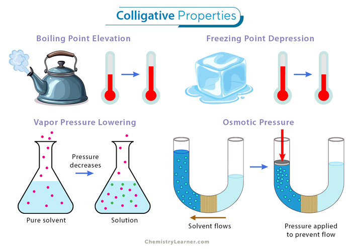
The four colligative properties are: [1-4]
Example
The following instances demonstrate colligative properties in solutions. When a small amount of salt is added to a glass of water, the solution’s freezing point significantly decreases compared to the water’s freezing point. Similarly, the solution’s boiling point rises, resulting in reduced vapor pressure. Moreover, alterations in the solution’s osmotic pressure also become evident.
Let us study briefly the abovementioned colligative properties.
1. Vapor Pressure Lowering
Every pure liquid exhibits a unique vapor pressure when in equilibrium with its liquid phase. The partial pressure associated with this equilibrium is intricately linked to temperature. In the case of solutions, their vapor pressure is notably lower than that of the pure solvent. The extent of this reduction depends upon the proportion of solute particles present, assuming the solute itself does not possess a substantial vapor pressure (nonvolatile).
The following formula gives the actual vapor pressure of a solution:
Psolution = χsolvent x Psolvent
Where:
– Psolution: Vapor pressure of the solution
– χsolvent: Mole fraction of the solvent
– Psolvent: Vapor pressure of the pure solvent
This equation is commonly referred to as Raoult’s law. The rationale behind vapor pressure depression is based on the assumption that solute particles occupy positions on the surface, displacing solvent particles. Consequently, this displacement hinders solvent evaporation.

2. Boiling Point Elevation
Due to the presence of a nonvolatile solute, the solution’s vapor pressure is lower than that of the pure solvent. A liquid boils when its vapor pressure becomes equal to the atmospheric pressure, which is 1 atm at sea level. To achieve this pressure, the solution must be at a higher temperature than the pure solvent’s boiling point.
The change in boiling point, denoted as ΔTb, can be easily computed using the formula:
ΔTb = i x Kb x m
Where:
– m is the molality
– Kb is the boiling point elevation constant
– i is the van’t Hoff factor

3. Freezing Point Depression
We have seen that the solution’s boiling point exceeds that of the pure solvent. However, an inverse effect is observed regarding the freezing point: The freezing point of the solution reduces below that of the pure solvent. This phenomenon can be visualized by considering how solute particles disrupt the cohesion of solvent particles during the formation of a solid, necessitating a lower temperature to induce solidification.
The change in freezing point (ΔTf) for a solution is given by:
ΔTf = i x Kf x m
Where:
– m is the molality
– Kf is the freezing point depression constant
– i is the van’t Hoff factor

4. Osmotic Pressure
Osmotic pressure is the pressure required to stop the spontaneous flow of solvent molecules through a semipermeable membrane from a region of lower solute concentration to one of higher solute concentration. It is a colligative property, meaning it depends on the number of solute particles in a solution, not their identity.
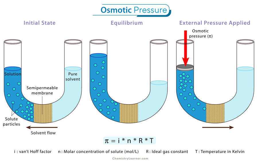
The osmotic pressure of a solution is mathematically expressed using the formula:
π = i x M x R x T
Where
– i: van’t Hoff factor
– M: molarity of the solution
– R: ideal gas constant
– T: absolute temperature (K)